In preparation for a deep learning course I’m taking over the Summer, I’m taking a short intro course on machine learning to help prepare me for some of the fundamental concepts. I’ve been avoiding AI for a while but given its ongoing application in nearly everything now, I figure it’s more than worth getting my feet wet.
ML Overview
Loss Functions
When we compare our predicted results to the actual results, how do we calculate the loss?
Loss functions can vary but they can be as simple as calculating the difference.
$$loss = sum(|y_{real} - y_{predicted}|)$$
$$loss = sum((y_{real} - y_{predicted})^2)$$
Datasets
- Training Set: Data to train the model
- Validation Set: Data that the model has not seen to ensure model can handle unseen data
- Testing Set: Data to test the model (seen or unseen)
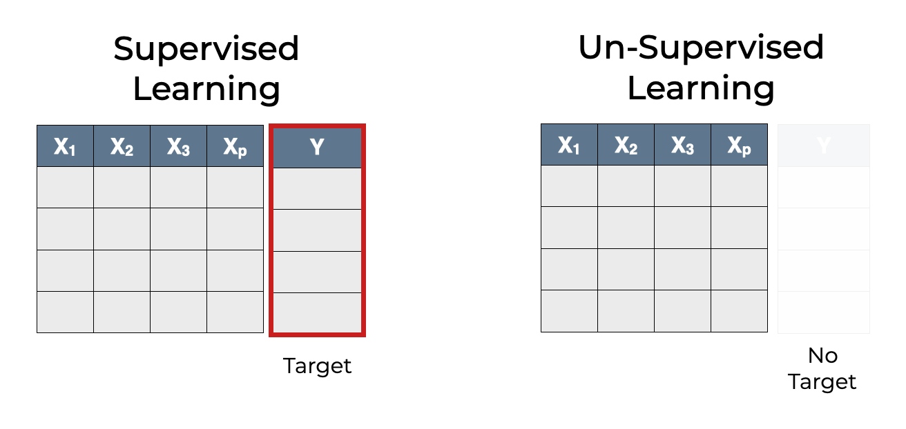
Types of Machine Learning
- Supervised Learning - Using labelled input data to train models, e.g. inputting animal pictured labelled with the coorresponding animal names.
- Unsupervised Learning - Using unlabelled input data to learn about pattern in data, e.g. inputting unlabelled animal pictures and having your machine try to group them
- Reinforcement Learning = Agent learning in an environment based on rewards and penalties
Supervised Learning
With a supervised dataset, you have a bunch of sampled data that each have an output label that classifies that data sample, as well as having 1 or more features which are just information about that subject.
For example you may be sampling for animals that are dogs, you’d have an output label dictating whether that simple is or isn’t a dog as well as features of the sample like their weight, size, and color.
We call the set of features the feature vector. We call the output label the target
Machine Learning Models
Once we have our data that we want to perform machine learning on, we need to decide on the model we use to classify new, unlabelled data.
K-Nearest Neighbours (KNN)
The intuition here is we have a labelled dataset, if get a new point in the dataset, we can infer how it should be labelled based on it’s distance from other points.
More formally, we take \(K\) of the nearest data points to our new point and based on the most common label, we infer the label of our new point. We can choose any number of \(K\) and depending on our dataset, can have varying levels of effectiveness.
Naive Bayes
Recall Bayes Theorem
$$ \def\series{x_1, x_2,…, x_n} P(A|B) = \frac{P(B|A)P(A)}{P(B)} $$
Naive Bayes is a generalization of this formula for a series of evidence.
For some category \(C_k\) (e.g. cats, dogs, etc.) and evidence \(\series\) (furry, red, small, etc.)
$$ P(C_k|\series)\ \alpha\ \Pi_{i=1}^n P(x_i|C_k)P(C_k) $$
- Our target acts as the category \(C_k\)
- Our feature vector act as the evidence \(\series\)
Derivation step for reference $$ P(C_k|\series)\ = \frac{P(\series|C_k)P(C_k)}{P(\series)} $$ Notice we remove the demoninator from Bayes Theorem. Since it isn’t influenced by \(C_k\), it acts as a constant. In following, \(\alpha\) stands for proportional since they are no longer equal.
But how do we use Naive Bayes to classify data?
$$\hat{y}\ (predicted\ category) = argmax_k P(C_k|\series)$$
We want to find the category that maximizes the probability given by the Naive Bayes. Essentially, we’ll be running Naive Bayes on each category and compare the categories that returns the highest probability.
Notice why Naive Bayes works despite only being a proportional value. We only want to compare probabilities, we don’t actually need the probability itself.
Logistic Regression

Support Vector Machines

Neural Network
For more complex data, modern approaches have been using neural network models.
The intuition of a neural network is that we want to break up our classification model into a set of neurons that take in
Equation for a Neuron
$$ \begin{bmatrix} x_0\\ x_1\\ \vdots\\ x_n \end{bmatrix} \cdot \begin{bmatrix} w_0\\ w_1\\ \vdots\\ w_n \end{bmatrix} \rightarrow z = \sum_{i} w_i x_i + b \rightarrow f(z) = a $$
Neurons & Hidden Layers

Neurons are grouped into layers known as hidden layers. We can have as many layers as deemed necessary, and each layer will have to job of classifying the data given by the previous layer.
For example, one layer may being classifying line strokes of an image while the next layer starts classifying different strokes together into shapes. The end goal may be to be able to identify text.
Weights & Biases
Each neuron’s job is to pick up on specific aspects of our input into it. They way we do this is by assigning weights to each of the inputs into the neuron.
For example, if our input is the pixels of a screen, perhaps we want our neuron to pick up only on a specific area on the screen of pixels. We would then have more postive weights on those pixels and weaker or potentially negative weights on the other pixels.
Every neuron will have it’s own associated weights that it assigns it’s inputs.
Depending on our data, we want our neuron to only be active at a certain magnitude of values. For instance, we want our neuron to start activating given a weighted sum > 10. The solution is adding a constant called a bias that shifts our sum so that it only activates at the values we want.
You might be wondering, “okay but, how do we decide these weight and biases?”. If we were to do this manually, it’d be an astronomical test of patience. Instead, the work of finding the right set of weights & biases will come later in the learning portion.
Activation Function
Once the weighted sums are calculated, they are run through an activation function as a final step before we take the value of that neuron.
Activation functions serve two primary purposes. Removing linearity from the network and for use in binary classification
Linearity in a network would mean multiple layers could just be represented as a single linear combination, removing the complexity of having multiple layers in the first place. Why does this help? Most phenomena in the world can’t be represented linearly and if they can, there’s likely not a need to use a neural net in the first place. We want to describe non-linear phenomena using a non-linear model.
As for the second purpose, the values from the weighted sums can be virtually anything but often we want them to be between 0 and 1. This is where an activation function can come in to add a final normalization to the value of a neuron.
A common activation function is the logistic function (sigmoid).
$$\sigma(x) = \frac{1}{1+e^{-x}}$$
This is almost exclusively used for output layers for the binary classification
A popular choice for hidden layer neurons is ReLU (Rectified Linear Unit)
$$ReLU(a) = max(0,a)$$
0 for a < 0, increases linearly otherwise
As an Equation
Luckily, this sequence of weighted sums, activations, and biases can be computed as a matrix.
$$ \def\activation{ a_0^{(1)} = \sigma( \begin{bmatrix} w_{0,0} & w_{0,0} & \dots & w_{0,n}\\ w_{0,0} & w_{0,0} & \dots & w_{0,n}\\ \vdots & \vdots & \ddots & \vdots \\ w_{k,0} & w_{k,0} & \dots & w_{k,n} \end{bmatrix} \begin{bmatrix} a_{0}^{(0)}\\ a_{1}^{(0)}\\ \vdots\\ a_{n}^{(0)} \end{bmatrix} + \begin{bmatrix} b_0\\b_1\\ \vdots \\b_n \end{bmatrix} ) } $$
Any single neuron \(a_n^{layer}\) is the combination of normalized (\(\sigma\)) weights and biases, of all the neurons from the previous layer.
Gradient Descent (or how calculus learns)
In order to start learning, we need an idea of how bad or good a particular set of weights and biases are. We call this the cost function.
The idea is that on every learning iteration, we want to minimize the cost function. However creating such a function and directly calculating some minimum isn’t a trivial task.
Instead, if we have some cost function, all we need to know is the slope of the function at a given input weights. Then we just need to shift the weights so that we move in the direction on the downward slope of the cost function. Hence, gradient descent.
Gradient descent just means walking in the downhill direction to minimize the cost function. - 3b1b

Back Propagation
This is the algorithm for efficiently computing gradient descent.
To reiterate, the goal of gradient descent is to systematically lower the cost function by adjusting the weights and biases for a given set of neurons.
A common cost function is to simply take the squared difference of the models prediction vs the actual values.
$$C(x) = (x - y)^2$$
The result is a series of values representing how closely or far away the model was the ideal answer.
Let’s however start our intuition with how would we want our outputs to change to get a lower cost. If we were trying to train our model to identify numbers, we would have outputs of all the digits 0-9. Now let’s say we give our model the number 2. Our ideal output is for the 2 output light up to one while every other output is zero. We’d likely want it to increase the weights & biases to lead to 2 as well as lower the weights & biases of all the other outputs.

Not only that, we out cost function, we know how far away each of our prediction are from the actual outputs. The more the cost, the more we want to lower or increase the weights & biases leading to that output.
Further more, we have 3 avenues to alter the activations for a neuron (the output of a neuron)
- Change the bias
- Change the weights
- Change the activations of the previous neuron
Recall the equation for the activation of a given neuron
$$\activation$$
Notice that we multiply the weights with the activations of the previous neurons. The brighter a neuron is, the more effect a change in weight will have. This is core to altering weights as we need to nudge them in proportion to the previous activations.
We can go through every one of the outcomes and collect an average of how much we want each of the preceeding neurons to change in order to get a better outcome. We can then repeat this for the previous layer’s neurons and so forth. Hence, back propagation.
In summary